import QuantLib as ql
import pandas as pd

today = ql.Date(2, ql.May, 2024)
ql.Settings.instance().evaluationDate = todayVanilla bonds
We’ve already seen in a previous notebook how to instantiate a fixed-rate bond. Here we expand on that: we’ll see a number of possible calculations, as well as other kinds of bonds that can be created and priced. Let’s start again from a sample fixed-rate bond and see what we can do.
schedule = ql.Schedule(
    ql.Date(8, ql.February, 2023),
    ql.Date(8, ql.February, 2028),
    ql.Period(6, ql.Months),
    ql.TARGET(),
    ql.Following,
    ql.Following,
    ql.DateGeneration.Backward,
    False,
)
settlement_days = 3
face_amount = 10_000
coupons = [0.03]
payment_day_counter = ql.Thirty360(ql.Thirty360.BondBasis)

bond = ql.FixedRateBond(
    settlement_days, face_amount, schedule, coupons, payment_day_counter
)
Static information
First of all, even without using an engine or other market data, the bond is able to return some static information. We can ask it for its current settlement date, or for the settlement date corresponding to another evaluation date:
print(bond.settlementDate())May 7th, 2024print(bond.settlementDate(ql.Date(31, ql.May, 2027)))June 3rd, 2027The same goes for the amount accrued so far: we can call the corresponding method without a date, returning the amount accrued up to the current settlement date, or pass another date. Note that the accrued amount, like prices, is scaled based on a notional of 100, not the actual face amount of the bond.
print(bond.accruedAmount())0.7416666666666627print(bond.accruedAmount(ql.Date(9, ql.May, 2027)))0.7583333333333275In this case, the passed date is treated as a settlement date; we can verify that this is the case by passing the current settlement date and checking that the returned amount equals the one returned by the call without date.
print(bond.accruedAmount(bond.settlementDate()))0.7416666666666627And for a further check, we can cycle over the next year and visualize the accrued amount at each date, verifying that it makes sense; that is, that it increases up to the full coupon amount and then resets to zero semiannually (the frequency of the bond we created.)
dates = [
    today + i for i in range(365) if ql.TARGET().isBusinessDay(today + i)
]
accruals = [bond.accruedAmount(d) for d in dates]

from matplotlib import pyplot as plt

ax = plt.figure(figsize=(9, 4)).add_subplot(1, 1, 1)
ax.plot([d.to_date() for d in dates], accruals, "-");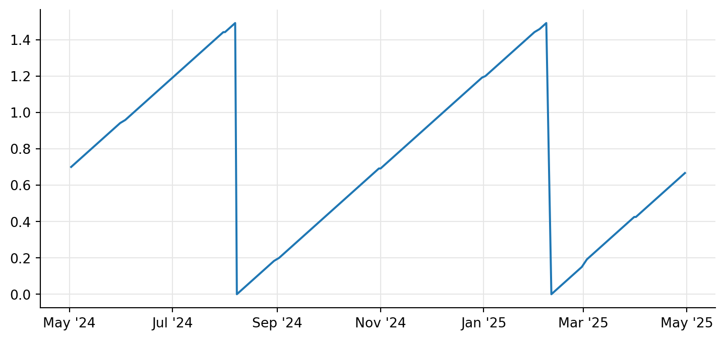
Cash flows
Again, we’ve already seen that we can perform cash-flow analysis on the bond. As a quick recap, the cashflows method returns a sequence of cash flows, each one providing basic information. In C++, the return type would be std::vector<shared_ptr<CashFlow>>, exported to Python as a list or tuple of CashFlow instances. As we’ve seen in another notebook, we can use helper functions to downcast them and perform a detailed cash-flow analysis, returning coupon-specific information when the cast succeeds and only basic information when it fails, as in the case of the bond redemptiom:
def coupon_info(cf):
    c = ql.as_coupon(cf)
    if not c:
        return (cf.date(), None, None, cf.amount())
    else:
        return (c.date(), c.rate(), c.accrualPeriod(), c.amount())


pd.DataFrame(
    [coupon_info(c) for c in bond.cashflows()],
    columns=("date", "rate", "accrual time", "amount"),
    index=range(1, len(bond.cashflows()) + 1),
).style.format({"amount": "{:.2f}", "rate": "{:.2%}"})| date | rate | accrual time | amount | |
|---|---|---|---|---|
| 1 | August 8th, 2023 | 3.00% | 0.500000 | 150.00 |
| 2 | February 8th, 2024 | 3.00% | 0.500000 | 150.00 |
| 3 | August 8th, 2024 | 3.00% | 0.500000 | 150.00 |
| 4 | February 10th, 2025 | 3.00% | 0.505556 | 151.67 |
| 5 | August 8th, 2025 | 3.00% | 0.494444 | 148.33 |
| 6 | February 9th, 2026 | 3.00% | 0.502778 | 150.83 |
| 7 | August 10th, 2026 | 3.00% | 0.502778 | 150.83 |
| 8 | February 8th, 2027 | 3.00% | 0.494444 | 148.33 |
| 9 | August 9th, 2027 | 3.00% | 0.502778 | 150.83 |
| 10 | February 8th, 2028 | 3.00% | 0.497222 | 149.17 |
| 11 | February 8th, 2028 | nan% | nan | 10000.00 |
Pricing
Calculating the price of the bond requires some market data, since we need to discount its cash flows. One way to do this is to use quoted yield information:
bond.cleanPrice(
    0.035,
    ql.Thirty360(ql.Thirty360.BondBasis),
    ql.Compounded,
    ql.Semiannual,
)98.25259209893974As I mentioned, the price is returned in base 100. At this time, there’s no support for bonds that are quoted in other units, e.g., around 1000 as some markets do.
Another way to calculate the price is to use a discount curve. Here I’ll use a simple flat rate for brevity, but any interest-rate term structure can be used; it could be, for instance, a Nelson-Siegel curve fitted on market prices. In this case, we’re not passing the discount curve to a bond method, as we did for the yield in the previous cell; instead, we pass it to a pricing engine and set the engine to the bond. This way, the bond will react if the curve changes. Additionally, we could keep hold of the term structure handle and relink it if necessary.
The engine we’re using is DiscountingBondEngine, which collects the dates and amounts from the cash flows, discounts them accordingly and accumulates them. (For more complex bonds, such as callables or convertibles, we’d need different engines.)
discount_curve = ql.FlatForward(0, ql.TARGET(), 0.04, ql.Actual360())
engine = ql.DiscountingBondEngine(
    ql.YieldTermStructureHandle(discount_curve)
)
bond.setPricingEngine(engine)
Once the pricing engine is set, we can ask the bond for its price and accrued amount without having to pass other arguments.
print(bond.cleanPrice())
print(bond.dirtyPrice())
print(bond.accruedAmount())
96.19296369916307
96.93463036582973
0.7416666666666627The usual NPV method is also implemented, but for bonds it can be confusing. Like dirtyPrice, it returns the cumulative discounted value of the cashflows; but it differs from dirtyPrice in a couple of points. First, its result is based on the face value of the bond; and second, it discounts the cash flows to the reference date of the discount curve (usually the global evaluation date) instead of the settlement date of the bond, as in the case of the price.
print(bond.NPV())9688.079274968233Note that the different discount date can matter more than one would expect; it means that, if a coupon is paid between the evaluation date and the settlement date of the bond, the coupon will be excluded from the dirty price but included in the NPV. We can see this by setting the evaluation date a business day before the date of the third coupon, August 8th 2024: after we normalize the NPV to the same units as the price, we can see a difference of about 1.5, corresponding to the coupon amount.
ql.Settings.instance().evaluationDate = ql.Date(7, 8, 2024)bond.dirtyPrice()96.48435372417977bond.NPV() / 10097.93059953484016In a way, you could see the dirty price as the value you would get from selling the bond (without considering tomorrow’s coupon, that you would receive before delivering the bond) and the NPV as the value you’d get from holding the bond until maturity (including tomorrow’s coupon).
This makes the NPV method useful in one particular case. When it’s too close to maturity, the bond can no longer price: for the sample bond we’re using, we’re still getting results one week before its maturity…
ql.Settings.instance().evaluationDate = ql.Date(1, 2, 2028)bond.cleanPrice()99.9882359483094…but a few days later, it returns a null price, even if the maturity has not been reached:
ql.Settings.instance().evaluationDate = ql.Date(4, 2, 2028)bond.cleanPrice()0.0This is because the settlement date is now at the maturity of the bond, and therefore the latter is no longer tradable.
print(bond.maturityDate())
print(bond.settlementDate())
February 8th, 2028
February 9th, 2028However, it’s still possible to calculate the NPV, which gives us the value of the cash flows still to receive.
bond.NPV()10144.656928164271Finally, and returning to the original evaluation date, it is also possible to obtain a yield from a price:
ql.Settings.instance().evaluationDate = today

print(
    bond.bondYield(
        ql.BondPrice(98.08, ql.BondPrice.Clean),
        ql.Thirty360(ql.Thirty360.BondBasis),
        ql.SimpleThenCompounded,
        ql.Semiannual,
    )
)0.03548806204795839(In C++ the method is called yield, but that’s a reserved keyword in Python.)
Duration and other figures
Some other calculations are not implemented as bond methods, but as static methods of the BondFunctions class; for instance, the various kinds of duration and the convexity.
print(
    ql.BondFunctions.duration(
        bond,
        0.035,
        ql.Actual360(),
        ql.Compounded,
        ql.Semiannual,
        ql.Duration.Macaulay,
    )
)3.6046062651997746print(
ql.BondFunctions.duration(
bond,
0.035,
ql.Actual360(),
ql.Compounded,
ql.Semiannual,
ql.Duration.Modified,
)
)3.542610580048918print(
ql.BondFunctions.convexity(
bond, 0.035, ql.Actual360(), ql.Compounded, ql.Semiannual
)
)14.76085604114641Other kinds of fixed-rate bonds
The same FixedRateBond class we used so far can also be instantiated with a sequence of several different coupon rates, making it possible to model step-up bonds:
schedule = ql.Schedule(
    ql.Date(8, ql.February, 2023),
    ql.Date(8, ql.February, 2028),
    ql.Period(6, ql.Months),
    ql.TARGET(),
    ql.Following,
    ql.Following,
    ql.DateGeneration.Backward,
    False,
)
settlement_days = 3
face_amount = 100
coupons = [0.03, 0.03, 0.04, 0.04, 0.05]
payment_day_counter = ql.Thirty360(ql.Thirty360.BondBasis)

bond = ql.FixedRateBond(
    settlement_days, face_amount, schedule, coupons, payment_day_counter
)
Here, as usual, we can see the corresponding cash flows.
pd.DataFrame(
    [coupon_info(c) for c in bond.cashflows()],
    columns=("date", "rate", "accrual time", "amount"),
    index=range(1, len(bond.cashflows()) + 1),
).style.format({"amount": "{:.2f}", "rate": "{:.2%}"})| date | rate | accrual time | amount | |
|---|---|---|---|---|
| 1 | August 8th, 2023 | 3.00% | 0.500000 | 1.50 |
| 2 | February 8th, 2024 | 3.00% | 0.500000 | 1.50 |
| 3 | August 8th, 2024 | 4.00% | 0.500000 | 2.00 |
| 4 | February 10th, 2025 | 4.00% | 0.505556 | 2.02 |
| 5 | August 8th, 2025 | 5.00% | 0.494444 | 2.47 |
| 6 | February 9th, 2026 | 5.00% | 0.502778 | 2.51 |
| 7 | August 10th, 2026 | 5.00% | 0.502778 | 2.51 |
| 8 | February 8th, 2027 | 5.00% | 0.494444 | 2.47 |
| 9 | August 9th, 2027 | 5.00% | 0.502778 | 2.51 |
| 10 | February 8th, 2028 | 5.00% | 0.497222 | 2.49 |
| 11 | February 8th, 2028 | nan% | nan | 100.00 |
To specify varying notionals, instead, we need to use the AmortizingFixedRateBond class:
schedule = ql.Schedule(
    ql.Date(8, ql.February, 2018),
    ql.Date(8, ql.February, 2028),
    ql.Period(1, ql.Years),
    ql.TARGET(),
    ql.Following,
    ql.Following,
    ql.DateGeneration.Backward,
    False,
)
settlement_days = 3
notionals = [10000, 10000, 8000, 8000, 6000, 6000, 4000, 4000, 2000, 2000]
coupons = [0.03]
payment_day_counter = ql.Thirty360(ql.Thirty360.BondBasis)

bond = ql.AmortizingFixedRateBond(
    settlement_days, notionals, schedule, coupons, payment_day_counter
)
bond.setPricingEngine(engine)
In this case, the cashflows include amortization payments:
pd.DataFrame(
    [coupon_info(c) for c in bond.cashflows()],
    columns=("date", "rate", "accrual time", "amount"),
    index=range(1, len(bond.cashflows()) + 1),
).style.format({"amount": "{:.2f}", "rate": "{:.2%}"})| date | rate | accrual time | amount | |
|---|---|---|---|---|
| 1 | February 8th, 2019 | 3.00% | 1.000000 | 300.00 |
| 2 | February 10th, 2020 | 3.00% | 1.005556 | 301.67 |
| 3 | February 10th, 2020 | nan% | nan | 2000.00 |
| 4 | February 8th, 2021 | 3.00% | 0.994444 | 238.67 |
| 5 | February 8th, 2022 | 3.00% | 1.000000 | 240.00 |
| 6 | February 8th, 2022 | nan% | nan | 2000.00 |
| 7 | February 8th, 2023 | 3.00% | 1.000000 | 180.00 |
| 8 | February 8th, 2024 | 3.00% | 1.000000 | 180.00 |
| 9 | February 8th, 2024 | nan% | nan | 2000.00 |
| 10 | February 10th, 2025 | 3.00% | 1.005556 | 120.67 |
| 11 | February 9th, 2026 | 3.00% | 0.997222 | 119.67 |
| 12 | February 9th, 2026 | nan% | nan | 2000.00 |
| 13 | February 8th, 2027 | 3.00% | 0.997222 | 59.83 |
| 14 | February 8th, 2028 | 3.00% | 1.000000 | 60.00 |
| 15 | February 8th, 2028 | nan% | nan | 2000.00 |
It’s also possible to ask for the current notional at a given date…
bond.notional(bond.settlementDate(ql.Date(25, 10, 2027)))2000.0…defaulting, as usual, to the current settlement date:
bond.notional()4000.0Following common market practice, the price returned by the class is scaled so that it’s in base 100 relative to the current notional; the NPV, as usual, returns the cash value. For instance:
bond.NPV()3910.55084058516bond.cleanPrice()97.07643264387757Zero-coupon bonds
There’s not a lot to say about these bonds; they can be instantiated by means of a dedicated class…
bond = ql.ZeroCouponBond(
    settlementDays=3,
    calendar=ql.TARGET(),
    faceAmount=10_000,
    maturityDate=ql.Date(8, ql.February, 2030),
)
bond.setPricingEngine(engine)
…and offer the same features of fixed-rate bonds.
print(bond.cleanPrice())79.162564713698print(
bond.bondYield(
ql.BondPrice(79.50, ql.BondPrice.Clean),
ql.Thirty360(ql.Thirty360.BondBasis),
ql.Compounded,
ql.Annual,
)
)0.040684510707855226print(
ql.BondFunctions.duration(
bond,
0.035,
ql.Actual360(),
ql.Compounded,
ql.Semiannual,
ql.Duration.Macaulay,
)
)5.841666666666667Floating-rate bonds
Not surprisingly, floating-rate bonds require an interest-rate index to determine the coupon rates; in turn, the index requires a forecasting curve. I’m using another flat curve for brevity, but in a real-world case it would probably be a curve bootstrapped from market data.
forecast_curve = ql.FlatForward(0, ql.TARGET(), 0.025, ql.Actual360())
euribor = ql.Euribor6M(ql.YieldTermStructureHandle(forecast_curve))
schedule = ql.Schedule(
ql.Date(8, ql.February, 2023),
ql.Date(8, ql.February, 2028),
ql.Period(6, ql.Months),
ql.TARGET(),
ql.Following,
ql.Following,
ql.DateGeneration.Backward,
False,
)
bond = ql.FloatingRateBond(
settlementDays=3,
faceAmount=10_000,
schedule=schedule,
index=euribor,
spreads=[0.001],
paymentDayCounter=ql.Actual360(),
paymentConvention=ql.Following,
)
bond.setPricingEngine(engine)Once instantiated, they provide the same facilities as fixed-rate bonds; however, they might also require a past index fixing to calculate the amount of the current coupon.
try:
    print(bond.cleanPrice())
except Exception as e:
    print(f"Error: {e}")
Error: Missing Euribor6M Actual/360 fixing for February 6th, 2024The missing fixings can be added through the index:
euribor.addFixing(ql.Date(6, ql.February, 2023), 0.028)
euribor.addFixing(ql.Date(4, ql.August, 2023), 0.0283)
euribor.addFixing(ql.Date(6, ql.February, 2024), 0.0279)

print(bond.cleanPrice())95.08004252605194Coupon and accrual information work the same (with future coupon rates and accruals being forecast via the curve, rather than determined). Once downcast, the coupons can provide a bit more information about the index fixings.
def coupon_info(cf):
    c = ql.as_floating_rate_coupon(cf)
    if not c:
        return (cf.date(), None, None, None, None, cf.amount())
    else:
        return (
            c.date(),
            c.fixingDate(),
            c.indexFixing(),
            c.rate(),
            c.accrualPeriod(),
            c.amount(),
        )


pd.DataFrame(
    [coupon_info(c) for c in bond.cashflows()],
    columns=(
        "payment date",
        "fixing date",
        "index fixing",
        "rate",
        "accrual time",
        "amount",
    ),
    index=range(1, len(bond.cashflows()) + 1),
).style.format(
    {"amount": "{:.2f}", "rate": "{:.2%}", "index fixing": "{:.2%}"}
)| payment date | fixing date | index fixing | rate | accrual time | amount | |
|---|---|---|---|---|---|---|
| 1 | August 8th, 2023 | February 6th, 2023 | 2.80% | 2.90% | 0.502778 | 145.81 |
| 2 | February 8th, 2024 | August 4th, 2023 | 2.83% | 2.93% | 0.511111 | 149.76 |
| 3 | August 8th, 2024 | February 6th, 2024 | 2.79% | 2.89% | 0.505556 | 146.11 |
| 4 | February 10th, 2025 | August 6th, 2024 | 2.52% | 2.62% | 0.516667 | 135.17 |
| 5 | August 8th, 2025 | February 6th, 2025 | 2.52% | 2.62% | 0.497222 | 130.05 |
| 6 | February 9th, 2026 | August 6th, 2025 | 2.52% | 2.62% | 0.513889 | 134.44 |
| 7 | August 10th, 2026 | February 5th, 2026 | 2.52% | 2.62% | 0.505556 | 132.25 |
| 8 | February 8th, 2027 | August 6th, 2026 | 2.52% | 2.62% | 0.505556 | 132.25 |
| 9 | August 9th, 2027 | February 4th, 2027 | 2.52% | 2.62% | 0.505556 | 132.25 |
| 10 | February 8th, 2028 | August 5th, 2027 | 2.52% | 2.62% | 0.508333 | 132.98 |
| 11 | February 8th, 2028 | None | nan% | nan% | nan | 10000.00 |
Also, floaters have a number of optional features; for instance, caps and floors. However, they require additional market information:
bond = ql.FloatingRateBond(
    settlementDays=3,
    faceAmount=10_000,
    schedule=schedule,
    index=euribor,
    paymentDayCounter=ql.Actual360(),
    paymentConvention=ql.Following,
    floors=[0.0],
    caps=[0.05],
)

bond.setPricingEngine(
    ql.DiscountingBondEngine(ql.YieldTermStructureHandle(discount_curve))
)try:
print(bond.cleanPrice())
except Exception as e:
print(f"Error: {e}")Error: pricer not setWhy is the error worded in this way? If you read the chapter on cash flows of Implementing QuantLib, you’ll see that floating-rate coupons (such as those created by the FloatingRateBond constructor) can be set a pricer, more or less like instruments can be set a pricing engine. We didn’t see it so far because, if caps and floors are not enabled, coupons based on an IBOR index are set a default pricer than calculates their fixing from the forecast curve they hold.
Caps and floors, however, introduce optionality and thus require volatility data. That information is missing from the default pricer, so the coupons are not given one during construction; we have to create the pricer ourselves and pass it to the coupons.
volatility = ql.ConstantOptionletVolatility(
    0, ql.TARGET(), ql.Following, 0.25, ql.Actual360()
)
pricer = ql.BlackIborCouponPricer(
    ql.OptionletVolatilityStructureHandle(volatility)
)
ql.setCouponPricer(bond.cashflows(), pricer)
print(bond.cleanPrice())94.68340203601055Looking at the cash flow information shows, for dates far enough in the future, that the effective rate paid by the coupon no longer equals the index fixing. This is due to the change in value coming from the caps and floors.
pd.DataFrame(
    [coupon_info(c) for c in bond.cashflows()],
    columns=(
        "payment date",
        "fixing date",
        "index fixing",
        "rate",
        "accrual time",
        "amount",
    ),
    index=range(1, len(bond.cashflows()) + 1),
).style.format(
    {"amount": "{:.2f}", "rate": "{:.4%}", "index fixing": "{:.4%}"}
)| payment date | fixing date | index fixing | rate | accrual time | amount | |
|---|---|---|---|---|---|---|
| 1 | August 8th, 2023 | February 6th, 2023 | 2.8000% | 2.8000% | 0.502778 | 140.78 |
| 2 | February 8th, 2024 | August 4th, 2023 | 2.8300% | 2.8300% | 0.511111 | 144.64 |
| 3 | August 8th, 2024 | February 6th, 2024 | 2.7900% | 2.7900% | 0.505556 | 141.05 |
| 4 | February 10th, 2025 | August 6th, 2024 | 2.5162% | 2.5162% | 0.516667 | 130.00 |
| 5 | August 8th, 2025 | February 6th, 2025 | 2.5159% | 2.5154% | 0.497222 | 125.07 |
| 6 | February 9th, 2026 | August 6th, 2025 | 2.5161% | 2.5136% | 0.513889 | 129.17 |
| 7 | August 10th, 2026 | February 5th, 2026 | 2.5159% | 2.5073% | 0.505556 | 126.76 |
| 8 | February 8th, 2027 | August 6th, 2026 | 2.5160% | 2.4976% | 0.505556 | 126.27 |
| 9 | August 9th, 2027 | February 4th, 2027 | 2.5159% | 2.4851% | 0.505556 | 125.64 |
| 10 | February 8th, 2028 | August 5th, 2027 | 2.5160% | 2.4707% | 0.508333 | 125.60 |
| 11 | February 8th, 2028 | None | nan% | nan% | nan | 10000.00 |
Floating-rate bonds on risk-free rates
There is no specific class yet for floaters that pay compounded overnight rates such as SOFR, ESTR or SONIA. However, it’s possible to create the cashflows and use them to build an instance of the base Bond class. The bond will figure out its redemption on its own.
forecast_curve = ql.FlatForward(0, ql.TARGET(), 0.02, ql.Actual360())
estr = ql.Estr(ql.YieldTermStructureHandle(forecast_curve))
As usual, the index will need past fixings. In the real world, you’d read them from a database or an API. Here, I’ll feed it constant ones for brevity:
d = ql.Date(8, ql.February, 2024)
while d < today:
    if estr.isValidFixingDate(d):
        estr.addFixing(d, 0.02)
    d += 1
Onwards with the bond construction:
schedule = ql.Schedule(
    ql.Date(8, ql.February, 2024),
    ql.Date(8, ql.February, 2029),
    ql.Period(1, ql.Years),
    ql.TARGET(),
    ql.Following,
    ql.Following,
    ql.DateGeneration.Backward,
    False,
)

coupons = ql.OvernightLeg(
    schedule=schedule,
    index=estr,
    nominals=[10_000],
    spreads=[0.0023],
    paymentLag=2,
)
In C++, the call to OvernightLeg above would be written as
Leg coupons =
    OvernightLeg(schedule, estr)
    .withNotionals(10000)
    .withSpreads(0.0023)
    .withPaymentLeg(2);
and, as you might guess, several other parameters are available. Finally, we can create the bond as
bond = ql.Bond(
    settlement_days,
    ql.TARGET(),
    schedule[0],
    coupons,
)
bond.setPricingEngine(engine)print(bond.cleanPrice())92.07577763235304This kind of bonds can also be used as a proxy for old-style floaters that need fall-back calculation after the cessation of LIBOR fixings.
A warning: duration of floating-rate bonds
If we try to pass a floating-rate bond we instantiated to the function provided for calculating bond durations, we run into a problem. For, say, a 1.5% semiannual yield, the result we get is:
forecast_curve = ql.FlatForward(0, ql.TARGET(), 0.015, ql.Actual360())
forecast_handle = ql.RelinkableYieldTermStructureHandle(forecast_curve)
euribor = ql.Euribor6M(forecast_handle)

schedule = ql.Schedule(
    ql.Date(8, ql.February, 2024),
    ql.Date(8, ql.February, 2028),
    ql.Period(6, ql.Months),
    ql.TARGET(),
    ql.Following,
    ql.Following,
    ql.DateGeneration.Backward,
    False,
)

bond = ql.FloatingRateBond(
    settlementDays=3,
    faceAmount=100,
    schedule=schedule,
    index=euribor,
    spreads=[0.001],
    paymentDayCounter=ql.Actual360(),
    paymentConvention=ql.Following,
)
y0 = 0.015
y = ql.InterestRate(y0, ql.Actual360(), ql.Compounded, ql.Semiannual)
print(ql.BondFunctions.duration(bond, y, ql.Duration.Modified))3.6491647768932602which is about the time to maturity. Shouldn’t we get the time to next coupon instead?
The problem is that the function above is too generic. It calculates the modified duration as \(\displaystyle{-\frac{1}{P}\frac{dP}{dy}}\); however, it doesn’t know what kind of bond it has been passed and what kind of cash flows are paid, so it can only consider the yield for discounting and not for forecasting. If you looked into the C++ code, you’d see that the bond price \(P\) above is calculated as the sum of the discounted cash flows, as in the following:
y = ql.SimpleQuote(y0)
yield_curve = ql.FlatForward(
    bond.settlementDate(),
    ql.QuoteHandle(y),
    ql.Actual360(),
    ql.Compounded,
    ql.Semiannual,
)

dates = [c.date() for c in bond.cashflows()]
cfs = [c.amount() for c in bond.cashflows()]
discounts = [yield_curve.discount(d) for d in dates]
P = sum(cf * b for cf, b in zip(cfs, discounts))

print(P)101.43285359570949Finally, the derivative \(\displaystyle{\frac{dP}{dy}}\) in the duration formula in approximated as \(\displaystyle{\frac{P(y+dy)-P(y-dy)}{2 dy}}\), so that we get:
dy = 1e-5

y.setValue(y0 + dy)
cfs_p = [c.amount() for c in bond.cashflows()]
discounts_p = [yield_curve.discount(d) for d in dates]
P_p = sum(cf * b for cf, b in zip(cfs_p, discounts_p))
print(P_p)

y.setValue(y0 - dy)
cfs_m = [c.amount() for c in bond.cashflows()]
discounts_m = [yield_curve.discount(d) for d in dates]
P_m = sum(cf * b for cf, b in zip(cfs_m, discounts_m))
print(P_m)

y.setValue(y0)
101.42915222219966
101.43655512613346print(-(1 / P) * (P_p - P_m) / (2 * dy))3.649164778159966which is, within accuracy, the same figure returned by BondFunctions.duration.
The reason is that the above doesn’t use the yield curve for forecasting, so it’s not really considering the bond as a floating-rate bond. It’s using it as if it were a fixed-rate bond, whose coupon rates happen to equal the current forecasts for the Euribor 6M fixings. This is clear if we look at the coupon amounts and discounts we stored during the calculation:
pd.DataFrame(
    list(zip(dates, cfs_p, discounts_p, cfs_m, discounts_m)),
    columns=(
        "date",
        "amount (+)",
        "discounts (+)",
        "amount (-)",
        "discounts (-)",
    ),
    index=range(1, len(dates) + 1),
)| date | amount (+) | discounts (+) | amount (-) | discounts (-) | |
|---|---|---|---|---|---|
| 1 | August 8th, 2024 | 1.461056 | 0.996144 | 1.461056 | 0.996149 |
| 2 | February 10th, 2025 | 0.829678 | 0.988478 | 0.829678 | 0.988493 |
| 3 | August 8th, 2025 | 0.798344 | 0.981155 | 0.798344 | 0.981180 |
| 4 | February 9th, 2026 | 0.825201 | 0.973644 | 0.825201 | 0.973679 |
| 5 | August 10th, 2026 | 0.811772 | 0.966311 | 0.811772 | 0.966355 |
| 6 | February 8th, 2027 | 0.811772 | 0.959033 | 0.811772 | 0.959087 |
| 7 | August 9th, 2027 | 0.811772 | 0.951810 | 0.811772 | 0.951873 |
| 8 | February 8th, 2028 | 0.816248 | 0.944602 | 0.816248 | 0.944674 |
| 9 | February 8th, 2028 | 100.000000 | 0.944602 | 100.000000 | 0.944674 |
You can see how the discount factors changed when the yield was modified, but the coupon amounts stayed the same.
Unfortunately, there’s no easy way to modify the BondFunctions.duration method so that it does what we expect. What we can do, instead, is to repeat the calculation above while setting up the bond and the curves so that the yield is used correctly. In particular, we have to link the forecast curve to the flat yield curve being modified; this might imply setting up a z-spread between forecast and discount curve, but I’ll gloss over this now. I’ll also set a pricing engine to the bond so it does the dirty price calculation for us.
forecast_handle.linkTo(yield_curve)
bond.setPricingEngine(
    ql.DiscountingBondEngine(ql.YieldTermStructureHandle(yield_curve))
)
y.setValue(y0 + dy)
P_p = bond.dirtyPrice()
cfs_p = [c.amount() for c in bond.cashflows()]
discounts_p = [yield_curve.discount(d) for d in dates]
print(P_p)
y.setValue(y0 - dy)
P_m = bond.dirtyPrice()
cfs_m = [c.amount() for c in bond.cashflows()]
discounts_m = [yield_curve.discount(d) for d in dates]
print(P_m)
y.setValue(y0)101.41322141911154
101.41375522190961Now the coupon amounts change with the yield (except, of course, the first coupon, whose amount was already fixed)…
pd.DataFrame(
    list(zip(dates, cfs_p, discounts_p, cfs_m, discounts_m)),
    columns=(
        "date",
        "amount (+)",
        "discounts (+)",
        "amount (-)",
        "discounts (-)",
    ),
    index=range(1, len(dates) + 1),
)| date | amount (+) | discounts (+) | amount (-) | discounts (-) | |
|---|---|---|---|---|---|
| 1 | August 8th, 2024 | 1.461056 | 0.996144 | 1.461056 | 0.996149 |
| 2 | February 10th, 2025 | 0.827280 | 0.988478 | 0.826247 | 0.988493 |
| 3 | August 8th, 2025 | 0.796037 | 0.981155 | 0.795043 | 0.981180 |
| 4 | February 9th, 2026 | 0.822816 | 0.973644 | 0.821788 | 0.973679 |
| 5 | August 10th, 2026 | 0.809426 | 0.966311 | 0.808415 | 0.966355 |
| 6 | February 8th, 2027 | 0.809426 | 0.959033 | 0.808415 | 0.959087 |
| 7 | August 9th, 2027 | 0.809426 | 0.951810 | 0.808415 | 0.951873 |
| 8 | February 8th, 2028 | 0.813889 | 0.944602 | 0.812872 | 0.944674 |
| 9 | February 8th, 2028 | 100.000000 | 0.944602 | 100.000000 | 0.944674 |
…and the duration is calculated correctly, approximating the four months to the next coupon.
print(-(1 / P) * (P_p - P_m) / (2 * dy))0.2631311153887885