import QuantLib as ql
import pandas as pd

today = ql.Date(25, ql.October, 2021)
ql.Settings.instance().evaluationDate = today

bps = 1e-4Curve bootstrapping
The process of bootstrapping, unlike fitting, uses an iterative algorithm to create a curve that reprices a number of instruments exactly. Each instrument, starting with the one with the shortest maturity, adds a node to the curve keeping the previous ones unchanged until the full curve is built.
When instruments need different curves, we can build them one by one, usually starting from the curve corresponding to the overnight index, e.g., SOFR in a US setting or ESTR in the Euro zone; this is because overnight-based instrument (usually futures and overnight-indexed swaps) only need that one curve, while other instruments need the overnight curve for discounting as well as other curves for forecasting.
In this notebook, I will provide a few short examples. However, there are lots of details that can be added; for a review of those (including, for instance, the possible addition of end-of-year jumps and synthetic instruments) you can read Ametrano and Bianchetti, Everything You Always Wanted to Know About Multiple Interest Rate Curve Bootstrapping but Were Afraid to Ask. A much longer notebook reproducing in Python the calculations in that paper is available on my blog.
Finally, Implementing QuantLib describes in detail the implementation of the algorithm, including the template machinery that makes it possible in C++ code to choose whether to interpolate discount factors, zero rates or instantaneous forwards, as well as to choose the kind of interpolation to be used, by declaring curves such as PiecewiseYieldCurve<Discount, LogLinear>, PiecewiseYieldCurve<ZeroYield, Linear> or PiecewiseYieldCurve<ForwardRate, BackwardFlat>.
And now, the examples.
Risk-free curves
These curves are used to forecast risk-free rates such as SOFR, SONIA or ESTR, as well as for risk-free discounting. In this case, I’ll use SOFR; of course, we have a class for that.
index = ql.Sofr()As I mentioned, the curve is built based on different kinds of instruments. The library defines helper classes corresponding to each of them, each instance acting as an objective function for the solver underlying the bootstrapping process.
For futures, the quote to reproduce is a price…
futures_data = [
    ((11, 2021, ql.Monthly), 99.934),
    ((12, 2021, ql.Monthly), 99.922),
    ((1, 2022, ql.Monthly), 99.914),
    ((2, 2022, ql.Monthly), 99.919),
    ((3, 2022, ql.Quarterly), 99.876),
    ((6, 2022, ql.Quarterly), 99.799),
    ((9, 2022, ql.Quarterly), 99.626),
    ((12, 2022, ql.Quarterly), 99.443),
]
…while for OIS, the quote is their fixed rate. In the list below, that shows quotes as they might come from some provider, the rates are in percent unit (that is, the 10-years rate is 1.359%); the library will require them in decimal units (i.e., 0.01359 for the same rate.)
ois_data = [
    ("1Y", 0.137),
    ("2Y", 0.409),
    ("3Y", 0.674),
    ("5Y", 1.004),
    ("8Y", 1.258),
    ("10Y", 1.359),
    ("12Y", 1.420),
    ("15Y", 1.509),
    ("20Y", 1.574),
    ("25Y", 1.586),
    ("30Y", 1.579),
    ("35Y", 1.559),
    ("40Y", 1.514),
    ("45Y", 1.446),
    ("50Y", 1.425),
]
Quotes are usually wrapped in SimpleQuote instances, so that they can be changed later; when this happens, the curve will then be notified and recalculate when needed. Once wrapped, they are passed to the helpers.
futures_helpers = []

for (month, year, frequency), price in futures_data:
    q = ql.SimpleQuote(price)
    futures_helpers.append(
        ql.SofrFutureRateHelper(ql.QuoteHandle(q), month, year, frequency)
    )
The above uses a specific helper, SofrFutureRateHelper, which knows how to calculate the relevant dates of SOFR futures given their month, year and frequency. It also knows that SOFR fixings are compounded in quarterly futures and averaged in monthly ones. For other indexes, for which no specific helper is available, it’s possible to use the OvernightIndexFutureRateHelper class instead; its constructor requires you to do a bit more work and pass it the start and end date of the underlying fixing period, as well as the averaging method to use.
The helper to use for OIS quotes is OISRateHelper; note that, as mentioned, the OIS rate is passed in decimal units, that is, 0.05 if the rate is 5%. In this case, I’m also saving the quotes in a map besides passing them to the helpers, so that I can access them more easily later on.
settlement_days = 2

ois_quotes = {}
ois_helpers = []

for tenor, quote in ois_data:
    q = ql.SimpleQuote(quote / 100.0)
    ois_quotes[tenor] = q
    ois_helpers.append(
        ql.OISRateHelper(
            settlement_days,
            ql.Period(tenor),
            ql.QuoteHandle(q),
            index,
            paymentFrequency=ql.Annual,
        )
    )
Another thing to note is that the ranges of futures and OIS can overlap; for instance, in this case, the maturity of the last futures is later than the maturity of the first OIS.
futures_helpers[-1].latestDate()Date(15,3,2023)ois_helpers[0].latestDate()Date(27,10,2022)In a real set of data, you would also have OIS quotes for maturities below the year. Using all the available helpers might cause collisions between maturities (which, in turn, would cause the bootstrap to fail); and even if that doesn’t happen, having nodes too close might result in unrealistic forwards between them. You’ll have to decide what to do: one possibility is to use only futures in the short range (since they’re usually more liquid) and start using swaps after the maturity of the last futures, possibly with a bit of buffer space, as in the cell below:
cutoff_date = futures_helpers[-1].latestDate() + ql.Period(1, ql.Months)
ois_helpers = [h for h in ois_helpers if h.latestDate() > cutoff_date]
Once the helpers are built and chosen, creating the curve is straightforward. There are a number of Python classes available (such as PiecewiseLogCubicDiscount, PiecewiseFlatForward, PiecewiseLinearZero and others), all wrapping the same underlying C++ class template with different arguments.
Creating the class doesn’t trigger bootstrapping, so the fact the the constructor succeeds doesn’t guarantee that the curve will work. The boostrapping code runs as soon as we call one of the methods of the curve to retrieve its results.
sofr_curve = ql.PiecewiseLogCubicDiscount(
    0,
    ql.UnitedStates(ql.UnitedStates.GovernmentBond),
    futures_helpers + ois_helpers,
    ql.Actual360(),
)
Depending on the chosen class, the nodes between which the curve interpolates will contain discount factors (as in this case), zero rates, or instantaneous forward rates.
pd.DataFrame(sofr_curve.nodes(), columns=["date", "discount factor"])| date | discount factor | |
|---|---|---|
| 0 | October 25th, 2021 | 1.000000 |
| 1 | December 1st, 2021 | 0.999933 |
| 2 | January 1st, 2022 | 0.999866 |
| 3 | February 1st, 2022 | 0.999792 |
| 4 | March 1st, 2022 | 0.999729 |
| 5 | June 15th, 2022 | 0.999378 |
| 6 | September 21st, 2022 | 0.998831 |
| 7 | December 21st, 2022 | 0.997888 |
| 8 | March 15th, 2023 | 0.996593 |
| 9 | October 27th, 2023 | 0.991743 |
| 10 | October 28th, 2024 | 0.979665 |
| 11 | October 27th, 2026 | 0.950236 |
| 12 | October 29th, 2029 | 0.902405 |
| 13 | October 27th, 2031 | 0.870431 |
| 14 | October 27th, 2033 | 0.840172 |
| 15 | October 27th, 2036 | 0.793002 |
| 16 | October 28th, 2041 | 0.724133 |
| 17 | October 29th, 2046 | 0.666582 |
| 18 | October 27th, 2051 | 0.617145 |
| 19 | October 27th, 2056 | 0.575211 |
| 20 | October 27th, 2061 | 0.544798 |
| 21 | October 27th, 2066 | 0.526100 |
| 22 | October 27th, 2071 | 0.496197 |
And just for kicks, we can visualize the curve we just created:
from matplotlib import pyplot as plt
from matplotlib.ticker import FuncFormatter
import numpy as np

ax = plt.figure(figsize=(9, 4)).add_subplot(1, 1, 1)
ax.yaxis.set_major_formatter(FuncFormatter(lambda r, pos: f"{r:.2%}"))
times = np.linspace(0.0, sofr_curve.maxTime(), 2500)
rates = [sofr_curve.zeroRate(t, ql.Continuous).rate() for t in times]
ax.plot(times, rates);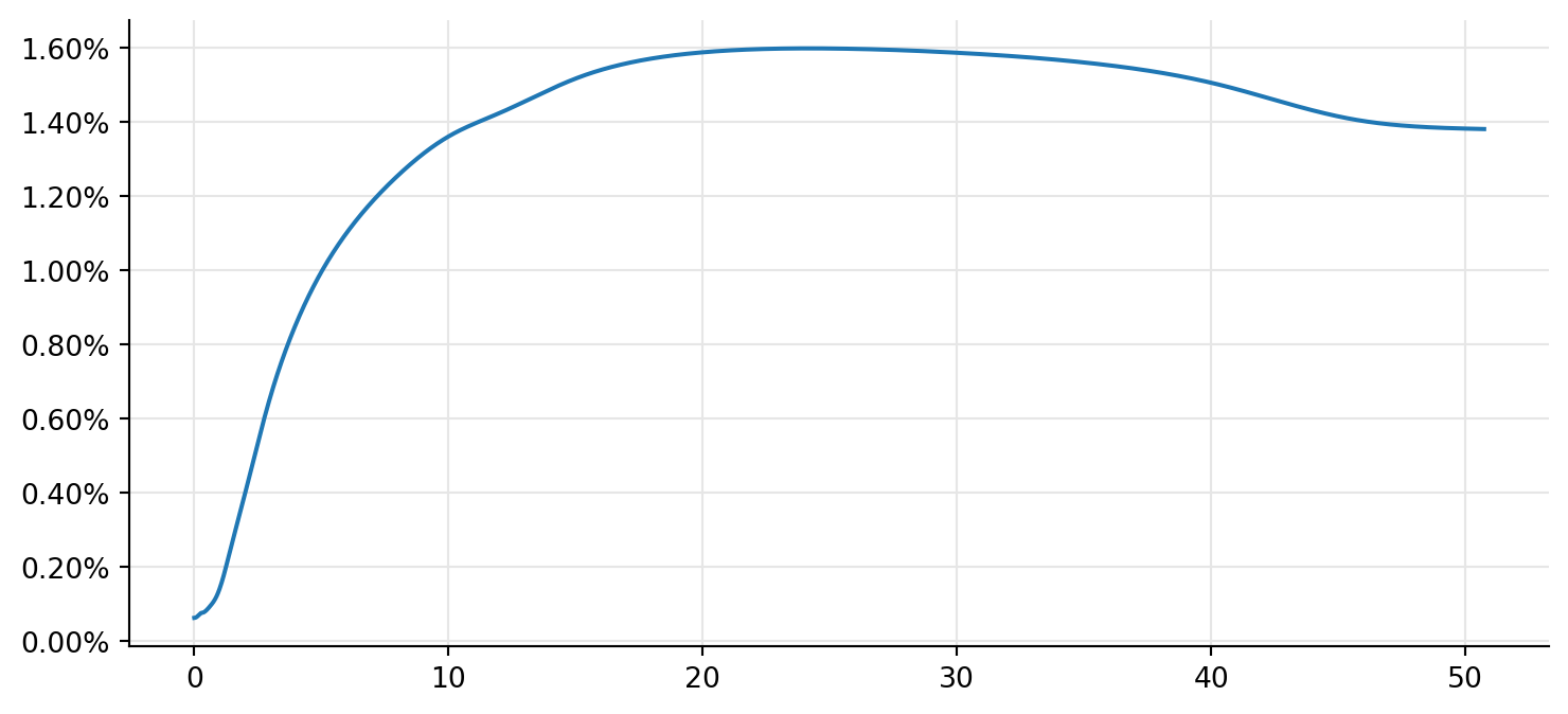
Checking the correctness of the curve
Having built the curve, one might be forgiven for not trusting us entirely and wanting to check the claim that it reprices the quotes exactly. The way to do it is to create the corresponding instruments and inspect them. For instance, to check the 20-years OIS quotes, we would create the corresponding swap and set the SOFR curve as its discounting curve; we also need to recreate the SOFR index so that it uses the same curve for forecasting.
sofr_handle = ql.YieldTermStructureHandle(sofr_curve)

index = ql.Sofr(sofr_handle)

start_date = index.fixingCalendar().advance(
    today, settlement_days, ql.Days
)
end_date = index.fixingCalendar().advance(
    start_date,
    ql.Period(20, ql.Years),
    index.businessDayConvention(),
    index.endOfMonth(),
)
schedule = ql.Schedule(
    start_date,
    end_date,
    ql.Period(ql.Annual),
    index.fixingCalendar(),
    index.businessDayConvention(),
    index.businessDayConvention(),
    ql.DateGeneration.Forward,
    index.endOfMonth(),
)

swap = ql.OvernightIndexedSwap(
    ql.Swap.Payer,
    1_000_000,
    schedule,
    0.0,
    index.dayCounter(),
    index,
)
swap.setPricingEngine(ql.DiscountingSwapEngine(sofr_handle))
Once we have the swap, we can ask for its fair rate and check that it equals the quoted OIS rate (1.574%) within numerical accuracy:
print(swap.fairRate())0.015739999999987143Modifying the curve as the quotes change
If you kept hold of the quotes like I did above, it’s also possible to modify any or all of them when market quotes change, or when you want to see the effect of a given change (more on this in another notebook.)
current_5y_value = ois_quotes["5Y"].value()
ois_quotes["5Y"].setValue(current_5y_value + 0.0010)

new_rates = [sofr_curve.zeroRate(t, ql.Continuous).rate() for t in times]

ois_quotes["5Y"].setValue(current_5y_value)
Here is the modified curve superimposed to the old one:
ax = plt.figure(figsize=(9, 4)).add_subplot(1, 1, 1)
ax.yaxis.set_major_formatter(FuncFormatter(lambda r, pos: f"{r:.2%}"))
ax.plot(times, rates, times, new_rates);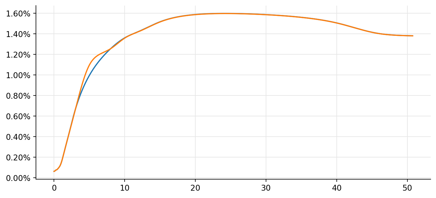
LIBOR curves
Actual LIBOR indexes were discountinued a while ago, but similar indexes such as Euribor remains; IBOR indexes, in library lingo. IBOR curves can be bootstrapped using quoted instruments based on the corresponding index; for instance, vanilla fixed-vs-floater swap.
swap_data = [
    (ql.Period("1y"), 0.417),
    (ql.Period("18m"), 0.662),
    (ql.Period("2y"), 0.863),
    (ql.Period("3y"), 1.185),
    (ql.Period("5y"), 1.443),
    (ql.Period("7y"), 1.606),
    (ql.Period("10y"), 1.711),
    (ql.Period("12y"), 1.742),
    (ql.Period("15y"), 1.804),
    (ql.Period("20y"), 1.856),
    (ql.Period("25y"), 1.896),
    (ql.Period("30y"), 1.932),
    (ql.Period("50y"), 1.924),
]
The vanilla-swap helpers use the curve being bootstrapped to forecast IBOR fixings, but according to current practice they take an external discount curve; here, in the interest of brevity, we’ll pretend that the SOFR curve we built above was really an ESTR curve. Of course, we should instead create a new one with the correct index, calendar and whatnot.
estr_curve = sofr_curveOnwards with the helpers. Vanilla swaps use the 6-months Euribor, so that’s the forecast curve we will bootstrap.
index = ql.Euribor(ql.Period(6, ql.Months))
settlement_days = 2
calendar = ql.TARGET()
fixed_frequency = ql.Annual
fixed_convention = ql.Unadjusted
fixed_day_count = ql.Thirty360(ql.Thirty360.BondBasis)

discount_handle = ql.YieldTermStructureHandle(estr_curve)

helpers = [
    ql.SwapRateHelper(
        ql.QuoteHandle(ql.SimpleQuote(quote / 100.0)),
        tenor,
        calendar,
        fixed_frequency,
        fixed_convention,
        fixed_day_count,
        index,
        ql.QuoteHandle(),
        ql.Period(0, ql.Days),
        discount_handle,
    )
    for tenor, quote in swap_data
]
The curve is built in the same way as the previous one:
euribor_6m_curve = ql.PiecewiseLinearZero(
    0, ql.TARGET(), helpers, ql.Actual360()
)
Again, we can look at its nodes (which, this time, contain zero rates…)
pd.DataFrame(
    euribor_6m_curve.nodes(), columns=["date", "rate"]
).style.format({"rate": "{:.4%}"})| date | rate | |
|---|---|---|
| 0 | October 25th, 2021 | 0.4106% |
| 1 | October 27th, 2022 | 0.4106% |
| 2 | April 27th, 2023 | 0.6512% |
| 3 | October 27th, 2023 | 0.8479% |
| 4 | October 28th, 2024 | 1.1626% |
| 5 | October 27th, 2026 | 1.4192% |
| 6 | October 27th, 2028 | 1.5815% |
| 7 | October 27th, 2031 | 1.6867% |
| 8 | October 27th, 2033 | 1.7169% |
| 9 | October 27th, 2036 | 1.7809% |
| 10 | October 28th, 2041 | 1.8344% |
| 11 | October 29th, 2046 | 1.8769% |
| 12 | October 27th, 2051 | 1.9172% |
| 13 | October 27th, 2071 | 1.8961% |
…and plot it, together with the ESTR curve:
ax = plt.figure(figsize=(9, 4)).add_subplot(1, 1, 1)
ax.yaxis.set_major_formatter(FuncFormatter(lambda r, pos: f"{r:.2%}"))
euribor_rates = [
    euribor_6m_curve.zeroRate(t, ql.Continuous).rate() for t in times
]
ax.plot(times, rates, times, euribor_rates);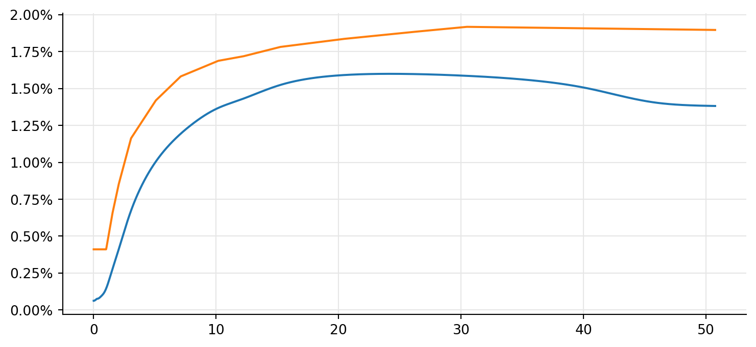
Quoted basis swaps
It is also possible to bootstrap a curve over quoted instruments such as OIS-vs-LIBOR swaps. For instance, we might have a set of quotes like this, in which we’re given the fair basis between the ESTR and Euribor legs in swaps with different maturities:
basis_data = [
    (ql.Period("1y"), 0.223),
    (ql.Period("18m"), 0.237),
    (ql.Period("2y"), 0.249),
    (ql.Period("3y"), 0.266),
    (ql.Period("5y"), 0.271),
    (ql.Period("7y"), 0.290),
    (ql.Period("10y"), 0.308),
    (ql.Period("12y"), 0.309),
    (ql.Period("15y"), 0.315),
    (ql.Period("20y"), 0.321),
    (ql.Period("25y"), 0.334),
    (ql.Period("30y"), 0.341),
    (ql.Period("50y"), 0.355),
]
In this case, we need to pass to the helpers (among other parameters) the ESTR index for the first leg, which needs to contain a forecast handle set to the ESTR curve…
estr = ql.Estr(ql.YieldTermStructureHandle(estr_curve))…and the Euribor index whose curve we want to bootstrap:
euribor3m = ql.Euribor(ql.Period(3, ql.Months))As before, we’ll build a helper for each quote. Some of the parameters are inferred from the passed indexes; for instance, the frequency of the payments (taken to be the same as the tenor of the LIBOR) and the day-count conventions, also taken for each coupon from the corresponding index. It is also possible to pass a discount curve, but if not, it is assumed to be the curve set to the overnight index.
settlement_days = 2
calendar = ql.TARGET()
convention = ql.ModifiedFollowing
end_of_month = False

helpers = [
    ql.OvernightIborBasisSwapRateHelper(
        ql.QuoteHandle(ql.SimpleQuote(quote / 100.0)),
        tenor,
        settlement_days,
        calendar,
        convention,
        end_of_month,
        estr,
        euribor3m,
    )
    for tenor, quote in basis_data
]
The curve is built as before:
euribor_3m_curve = ql.PiecewiseLogCubicDiscount(
    0, ql.TARGET(), helpers, ql.Actual360()
)
ax = plt.figure(figsize=(9, 4)).add_subplot(1, 1, 1)
ax.yaxis.set_major_formatter(FuncFormatter(lambda r, pos: f"{r:.2%}"))
euribor_rates = [
euribor_3m_curve.zeroRate(t, ql.Continuous).rate() for t in times
]
ax.plot(times, rates, times, euribor_rates);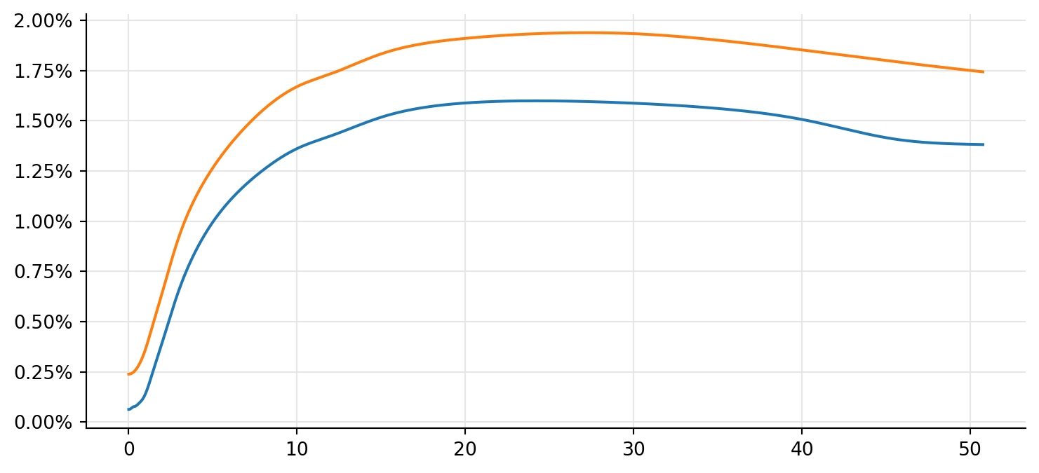
It is also possible to bootstrap a curve over a mix of vanilla and basis swaps, provided that they’re based on the same IBOR index.
Swap pricing
Once the relevant curves are built, it’s possible to price swaps; for instance, a fixed-vs-Euribor swap. First, we build the Euribor index and pass it the corresponding forecast curve:
forecast_handle = ql.YieldTermStructureHandle(euribor_6m_curve)

euribor6m = ql.Euribor(ql.Period(3, ql.Months), forecast_handle)
Then we build the swap, passing the conventions and terms it needs:
start_date = ql.Date(18, ql.November, 2021)
end_date = start_date + ql.Period(30, ql.Years)
fixed_coupon_tenor = ql.Period(ql.Annual)
calendar = ql.TARGET()
rule = ql.DateGeneration.Forward
float_convention = ql.ModifiedFollowing
end_of_month = False
fixed_rate = 150 * bps
floater_spread = 10 * bps

fixed_schedule = ql.Schedule(
    start_date,
    end_date,
    fixed_coupon_tenor,
    calendar,
    fixed_convention,
    fixed_convention,
    rule,
    end_of_month,
)
float_schedule = ql.Schedule(
    start_date,
    end_date,
    euribor6m.tenor(),
    calendar,
    float_convention,
    float_convention,
    rule,
    end_of_month,
)
swap = ql.VanillaSwap(
    ql.Swap.Payer,
    1_000_000,
    fixed_schedule,
    fixed_rate,
    fixed_day_count,
    float_schedule,
    euribor6m,
    floater_spread,
    euribor6m.dayCounter(),
)
Finally, we tell its pricing engine to use the ESTR curve for discounting:
swap.setPricingEngine(ql.DiscountingSwapEngine(discount_handle))We can now ask the swap for its value, or other figures:
swap.NPV()128295.50732521049swap.fairRate()0.02037361224452942Jumps
If you have a forecast of a future jump in rates (such as those that may happen an the end of an year, or in correspondence of ECB meeting dates, or others) it’s possible to include it in the bootstrapped curve.
Let’s go back to the SOFR curve, and let’s assume that we estimated an end-of-year jump of 15 basis points at the end of next December. (Here, we’ll pull it out of thin air; for an example of its calculation, you can see the Ametrano-Bianchetti paper and notebook I linked above.)
index = ql.Sofr()jump_date = ql.Date(31, ql.December, 2021)
J = 0.0015A slight snag is that the curve doesn’t expect jumps to be expressed as an increase in rates (\(J\) above), but as a corresponding additional discount factor \(B = 1 / (1 + J \tau)\) where \(\tau\) is the horizon of the jump; in this case, from the jump date to the next business day.
tau = sofr_curve.dayCounter().yearFraction(
    jump_date, index.fixingCalendar().advance(jump_date, 1, ql.Days)
)
B = 1 / (1 + J * tau)
We can now create a new curve, bootstrapped over the same helpers as the original SOFR curve but including the jump. The curve can manage multiple jumps, which is the reason why the jump and its date are both passed as a list of one element.
sofr_curve_j = ql.PiecewiseLogCubicDiscount(
    0,
    ql.UnitedStates(ql.UnitedStates.GovernmentBond),
    futures_helpers + ois_helpers,
    ql.Actual360(),
    [ql.makeQuoteHandle(B)],
    [jump_date],
)
We can see the effect of the jump on the curve by plotting the short end (say, within one year from today) of both the old and new curve:
calendar = index.fixingCalendar()
dates = calendar.businessDayList(today, today + ql.Period(12, ql.Months))

rates = [
    sofr_curve.zeroRate(d, index.dayCounter(), ql.Continuous).rate()
    for d in dates
]
new_rates = [
    sofr_curve_j.zeroRate(d, index.dayCounter(), ql.Continuous).rate()
    for d in dates
]

ax = plt.figure(figsize=(9, 4)).add_subplot(1, 1, 1)
ax.yaxis.set_major_formatter(FuncFormatter(lambda r, pos: f"{r:.2%}"))
ax.plot([d.to_date() for d in dates], rates, label="without jump")
ax.plot([d.to_date() for d in dates], new_rates, label="with jump")
ax.legend(loc="best");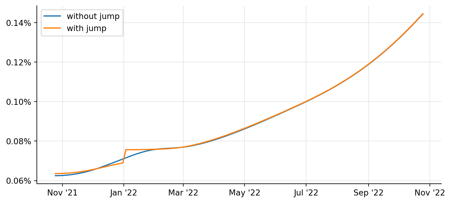
The jump is clearly visible, as well as the fact that the rates around the jump also change so that the curve still reprices the quoted instruments exactly.